Chapter 3 Data
You can skip this chapter if you:
-
Are comfortable working with dataframes and tibbles
-
Know about and are comfortable using some of R’s inbuilt data packages
-
Are comfortable loading .csv and .xlsx files into R
3.1 Packages for this chapter
In this chapter you’ll want the following packages loaded in your R session. At the start, you will need to run the following code. Remember if you don’t have a package you can install it with the install.package("package_name") command.
3.2 Built In Data
Many packages, such as the tidyverse package, and the default 3 datasets package come with data in them. These datasets can be really useful for testing code that you’re unfamiliar with, because you know what the data should look like, and how it should perform.
Some common datasets are:
mpg- Fuel economy data from 1999 to 2008 for 38 popular models of cars
ChickWeight- Weight versus age of chicks on different diets
starwars- Name, height, weight, age, and other characteristics of Star Wars characters
iris- The measurements (in cm) of the sepal length and width and petal length and width of 50 flowers in 3 species of iris
There are many, many more. You can explore some of them by typing datasets:: into the console and instead of pressing ‘enter’, scroll the menu that pops up to help you autocomplete your command.
You might wonder, what’s the :: in the
datasets:: command. The :: is very useful and
tells R to look inside the datasets package without having
to actually load it into your library which can be very quick and
easy.
But be careful! If you are sharing your code with lots of other people, this can sometimes make it a bit harder for other people to run your code. This is called ‘environment management’ and something you’ll learn more about as your R journey continues.
3.3 Exercise
For our first exercise we are going to look at some of the inbuilt datasets.
What happens when you enter the following code4 into the console?
You should see something like Figure 3.1
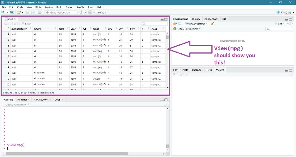
Figure: 3.1: The result of the ‘View(mpg)’ command
The View() command is very handy for getting a quick window onto what data looks like. Unfortunately, the View() command only really works for you getting a look at your data. If you wanted to share your code, you would be better using a command which prints some of the data into the console.
So - what functions will tell R to print data into the console?
You can view the top of a dataset with head()
## # A tibble: 6 × 11
##   manufacturer model displ  year   cyl trans      drv     cty   hwy fl    class
##   <chr>        <chr> <dbl> <int> <int> <chr>      <chr> <int> <int> <chr> <chr>
## 1 audi         a4      1.8  1999     4 auto(l5)   f        18    29 p     compact
## 2 audi         a4      1.8  1999     4 manual(m5) f        21    29 p     compact
## 3 audi         a4      2    2008     4 manual(m6) f        20    31 p     compact
## 4 audi         a4      2    2008     4 auto(av)   f        21    30 p     compact
## 5 audi         a4      2.8  1999     6 auto(l5)   f        16    26 p     compact
## 6 audi         a4      2.8  1999     6 manual(m5) f        18    26 p     compact
Note that this code has produced an output block. Unlike View() where I had to share a screengrab to show you what the output of the code was. This is why head() is a lot more reproducible than View() and should be your default for code sharing. See more about this in workflows.
Unsurprisingly we can also view the bottom of a dataset with …
## # A tibble: 6 × 11
##   manufacturer model  displ  year   cyl trans      drv     cty   hwy fl    class
##   <chr>        <chr>  <dbl> <int> <int> <chr>      <chr> <int> <int> <chr> <chr>
## 1 volkswagen   passat   1.8  1999     4 auto(l5)   f        18    29 p     midsize
## 2 volkswagen   passat   2    2008     4 auto(s6)   f        19    28 p     midsize
## 3 volkswagen   passat   2    2008     4 manual(m6) f        21    29 p     midsize
## 4 volkswagen   passat   2.8  1999     6 auto(l5)   f        16    26 p     midsize
## 5 volkswagen   passat   2.8  1999     6 manual(m5) f        18    26 p     midsize
## 6 volkswagen   passat   3.6  2008     6 auto(s6)   f        17    26 p     midsize
Another very useful way to look at a dataset is with the summary() function, which takes its best guess at how to summarise each variable in the dataset.
##  manufacturer          model               displ            year           cyl           trans               drv
##  Length:234         Length:234         Min.   :1.600   Min.   :1999   Min.   :4.000   Length:234         Length:234
##  Class :character   Class :character   1st Qu.:2.400   1st Qu.:1999   1st Qu.:4.000   Class :character   Class :character
##  Mode  :character   Mode  :character   Median :3.300   Median :2004   Median :6.000   Mode  :character   Mode  :character
##                                        Mean   :3.472   Mean   :2004   Mean   :5.889
##                                        3rd Qu.:4.600   3rd Qu.:2008   3rd Qu.:8.000
##                                        Max.   :7.000   Max.   :2008   Max.   :8.000
##       cty             hwy             fl               class
##  Min.   : 9.00   Min.   :12.00   Length:234         Length:234
##  1st Qu.:14.00   1st Qu.:18.00   Class :character   Class :character
##  Median :17.00   Median :24.00   Mode  :character   Mode  :character
##  Mean   :16.86   Mean   :23.44
##  3rd Qu.:19.00   3rd Qu.:27.00
##  Max.   :35.00   Max.   :44.00
The summary() function highlights an important aspect of R - it knows the difference between numbers and characters. In the output block we can see that manufacturer is given the Class character. R knows it can’t create a mean and a median from this data, so it simply tells you the Length of that data instead. What do you think the 234 refers to here? Answer in the footnote5.
3.4 Data you create
Sometimes you will want to test something on pretend data, or run something on a very small dataset. In these cases, we can create a dataset in our environment. This can be really useful for troubleshooting because you can create data that shows your problem, and this is easier to share with others.
For example, lets say we we were interested in this idea that R only sees manufacturer in mpg as a string of letters. How can we tell R that manufacturer is in fact a category? We can test on a smaller, simpler dataset.
3.5 Exercise - Creating data
We are going to use a new function here called tibble which will make a dataframe quickly and easily. Before when we were typing things like x <- 1, we created a single thing in the environment. Now we want to create multiple thing (rows and columns) and that’s what the tibble function will do.
Try the following and watch what happens in your environment (you’ll need the tidyverse loaded - see above)
You can View(dat) to look at this (or use head(dat)). Let’s try and replicate our weird summary(mpg) character issue.
##        x             y
##  Min.   :1.00   Length:6
##  1st Qu.:2.25   Class :character
##  Median :3.50   Mode  :character
##  Mean   :3.50
##  3rd Qu.:4.75
##  Max.   :6.00
We can replicate the issue. You can see that the y variable has the class: Character. What can we do about it?
We essentially want to tell R that y is not a character, but a factor6.
We can ask R more directly what y is by telling it exactly where to look.
## [1] TRUEThe $ symbol tells R that it needs to look inside dat for y. Try typing out is.character(y) or is.character(dat::y) and see what happens. What are those error messages telling you? 7
If the is.character() function asks R if the named object is a character, how do you think we ask R if the named object is a factor? Try typing out your answer in the console to see what happens.
We therefore need to ask R to change the data. We can do this like so:
## [1] A B A B A B
## Levels: A B
And we get a response. But what happens if we run summary(dat) again?
##        x             y
##  Min.   :1.00   Length:6
##  1st Qu.:2.25   Class :character
##  Median :3.50   Mode  :character
##  Mean   :3.50
##  3rd Qu.:4.75
##  Max.   :6.00
Why do you think this happens?
You should take time to stop and answer these questions before reading on - practice and thinking about R is the best way to learn.
It happens because we haven’t actually changed the data. With as.factor(dat$y), R told us the answer, but didn’t edit the object in any way. To change the dat dataframe, we need to use the assign (<-) function to make sure R saves it into the environment.
Here’s the fun part. We can do this in two (or actually - many) different ways. In a lot of ways, its personal preference which one you choose . . .
To demonstrate, we will make two new dataframes.
Option 1
Option 2
In Option 1, we are essentially saying something like:
-
Make a new thing called
option1 -
That thing is a tibble
-
That tibble should contain x, from dat (
dat$x) -
That tibble should contain y, from dat, made into a factor (
as.factor(dat$y))
Whereas in Option 2, we are saying:
-
Make an new thing caled
option2 -
That thing should start the same as
dat -
We use the pipe command (
|>) to say ‘and then’ -
So take
datand then change something indat(themutatefunction) -
Make y a factor (
y = as.factor(y))
With Option 2, we don’t need to specify dat$y because we are using the pipe function (|>) to tell R we are still working with the dat dataframe.
The |> pipe is a relatively recent implementation, but tidyverse has utilised the %>% pipe from the magrittr package for years. Lots of documentation will use the magrittr pipe %>% online, and even in this book. Either is fine and should both work in any cases. (There are a few special cases where they function differently which Hadley Wickham talks about here)
Personally, I found the pipe function in tidyverse to be revolutionary when I learned it, and its by far my favourite way to write code. I find the code in Option 2 a lot easier to read than the code in Option 1, and we’ll be using tidyverse in the rest of this book. However, here’s another important thing:
You do not have to code like I do - so long as I can run your code, we don’t have to approach a problem in the same way.
This will become clearer as we work through the book.
To test that we have done what we wanted to do - let’s run the summary() function again.
##        x        y
##  Min.   :1.00   A:3
##  1st Qu.:2.25   B:3
##  Median :3.50
##  Mean   :3.50
##  3rd Qu.:4.75
## Max. :6.00## x y
## Min. :1.00 A:3
## 1st Qu.:2.25 B:3
## Median :3.50
## Mean :3.50
## 3rd Qu.:4.75
## Max. :6.00And now we see that R has changed y into a factor, both ways, and now we have a different output to the summary() function.
Thinking back to our mpg example - can you change the mpg dataset so that manufacturer is a factor?
Can you change multiple variables to factors?
Is
tidyverseor base R easier to use for changing multiple factors?If you google, do you find other ways of changing
mpg?
Once you have tried these - you can view some of my answers here
3.6 Loading data from your hard drive
Finally, sometimes you will have data delivered to you on a file that you will want to load in to R. These will usually be *.csv or *.xlsx files
These can easily be read in with a function. The most commonly used function for *.csv files is read.csv. For excel files its read_excel from the readxl package. There are also ways to load data from URLs, and word documents, and all sorts!
The skill most needed to load files from your hard drive is the ability to navigate and understand folder structures (sometimes called working directories). If your desktop has a hundred files then you should go and watch this video.
We will use two different files for the rest of this chapter.
You should download the two files and save them into the folder you are using for your R Project. We will explore directories a bit in the next section, but its better to start good practice now.
The two files are:
-
ch2_planets.xlsx
-
ch2_planets.csv
You will find them on your Learn course under this week’s materials.
If you are learning independently, you will also find them in the data folder on my github page.
3.7 Loading data
3.7.1 Loading from a CSV
There are two main ways to load a .csv file.
The easy way is to navigate to the environment tab and click on Import Dataset
Scroll down to From Text (base) and click through the import wizard, navigating to where you saved your file.
Here is a short demonstration:
Figure: 3.2: Using the Import Dataset wizard to load a csv file
Note that the the import wizard runs code in the console which says something like:
If you copy this code you can run it yourself. You know by now that anything to the left of the assign command (<-) is the name of the thing you’re creating.
3.8 Exercise
Change this code so you’re creating a dataset called dat not ch2_planets. Answer here
3.8.1 Loading from an Excel file
Similar to above, you can upload an .xlsx file in two different ways, using the wizard, or by typing in the code.
To use the wizard, you again navigate to the environment tab and click on Import Dataset
Scroll down to From Excel and click through the import wizard, navigating to where you saved your file. Depending on what your excel file looks like
Here is a short demonstration:
Figure: 3.3: Using the Import Dataset wizard to load a xlsx file
This time, note that the console first loads a package (library(readxl)) before it loads the data.
Again you can copy this code and run the code itself in an R Script file, in a R Markdown file, or in the console, to load the data without going through the wizard.
Why would you want to use code instead of the wizard?
We will come to talk about repeatable workflows in a later chapter, but basically - if you send me an R Script file with the code for loading in the data, I can run that file without having to edit it.
You can send me your script and your data file together, and I can work directly on it, which saves a huge amount of time and makes collaborating easier.
3.9 Exercise
This time I want you to load the ch2_planets.xlsx file into your environment.
I assume that you have saved the ch2_planets.xlsx file to your working directory in a folder called data.
Your task: I don’t want to have to load the readxl library every time I read in an excel file. Is there a short cut we can use?
Remember to try this - play about with the code and talk to your classmates/friends before looking at the answer. Answer here
‘Default’ here means one you won’t need to install or load into the library↩︎
If its not working - are you sure you have spelled it with a capital
View?↩︎The Length of these variables is the number of rows in each one, which for this case is the same for each variable because this is a nice, tidy dataset↩︎
A factor is also called a categorical variable, or a grouping variable. If you’re not sure you know what a factor is, wiki is a good place to review↩︎
is.character(y)should give you an error message likeError: object 'y' is not foundbecauseyby itself does not exist in your environment. There’s a way around this by ‘attaching’ data to your environment, which is a bit old fashioned and can result in problems down the line with your workflow (because you won’t necessarily know if the person you’re working with has also attached the data), so I recommend against it.is.character(dat::y)should give you an error likeError in loadNamespace(name) : there is no package called 'dat'. Unsurprisingly, this is telling you that the::sequence tells R to look inside a package for a thing calledy, but that package doesn’t exist. Packages and data frames are different things.↩︎