Chapter 14 Answers

14.1 Creating Data Answers

Here are the answers to Creating Data

14.1.1 Changing mpg data

Changing one variable is pretty easy to do in tidyverse:

mpg2 <- mpg |> 
  mutate(manufacturer = as.factor(manufacturer))

But what if we want to change all the character variables?

We can still use mutate like this:

mpg2 <- mpg |> 
  mutate(manufacturer = as.factor(manufacturer),
         model = as.factor(model),
         trans = as.factor(trans),
         drv = as.factor(drv),
         fl = as.factor(fl),
         class = as.factor(class))

Or we can use a slightly different command to apply the as.factor function across selected variables, predictably called mutate_at()

mpg2 <- mpg |> 
  mutate_at(.vars = vars(c(manufacturer, model, trans, drv, fl, class)),
            .funs = as.factor)

mutate_at becomes a very useful way of shortening your code, but can also be a little bit more difficult to remember. I very often have to look it up. But that’s fine - looking up code is good :)

14.2 Loading csv data answers

Here’s the answer to how to change the name of a dataset from a csv file

dat <- read.csv("~/data/ch2_planets.csv")

Here is a chunk of text to hide the next answer from you in case you’re doing these answers sequentially.

Figure: 14.1: Using the Import Dataset wizard to load a xlsx file

14.3 Loading excel data answers

In this section I asked you to load data from a different folder and have a short cut to stop us having to load readxl each time

If the below code doesn’t make sense to you - reach out to me!

dat <- readxl::read_excel("data/ch2_planets.xlsx")

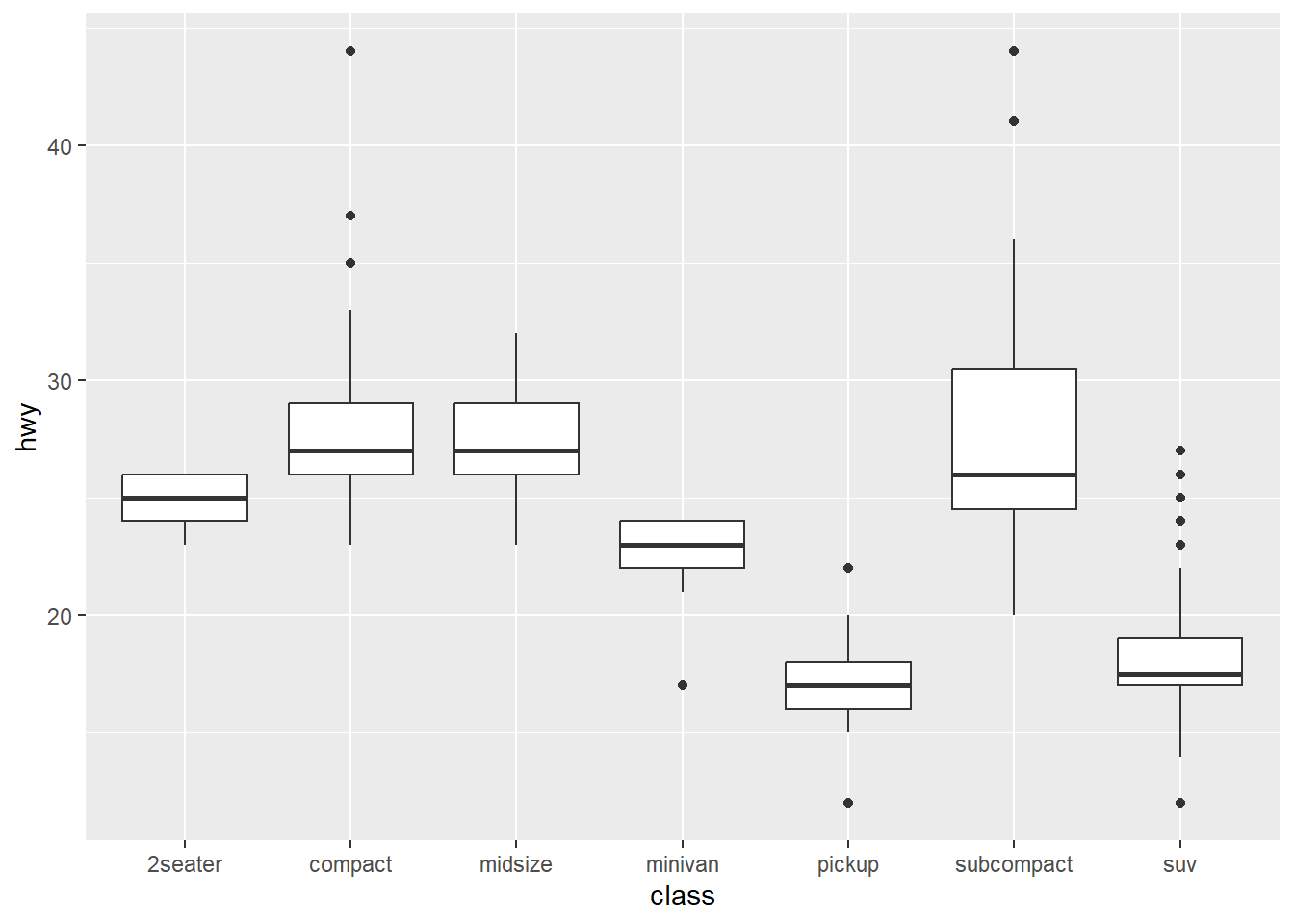
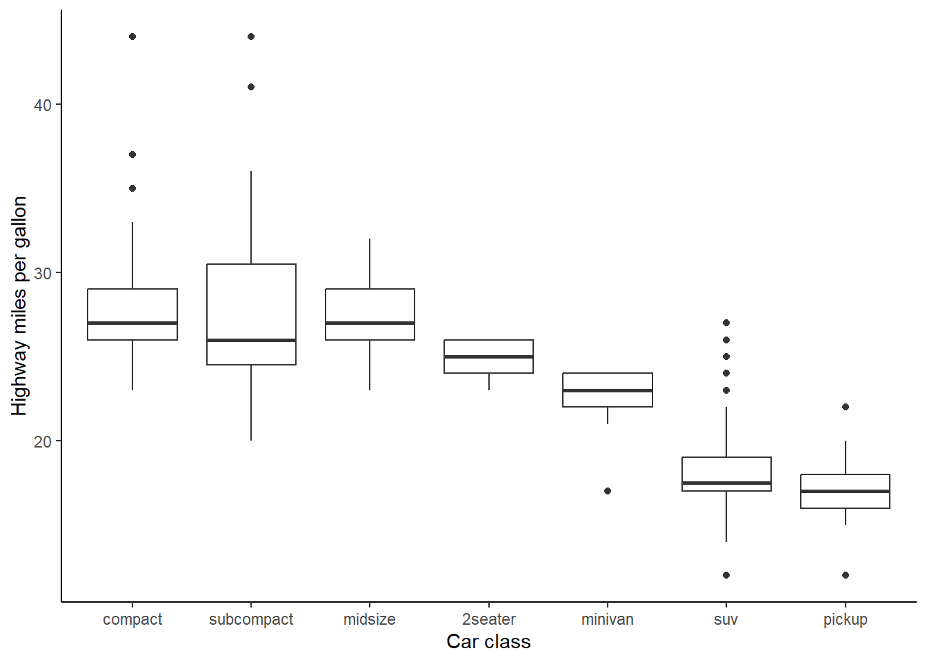
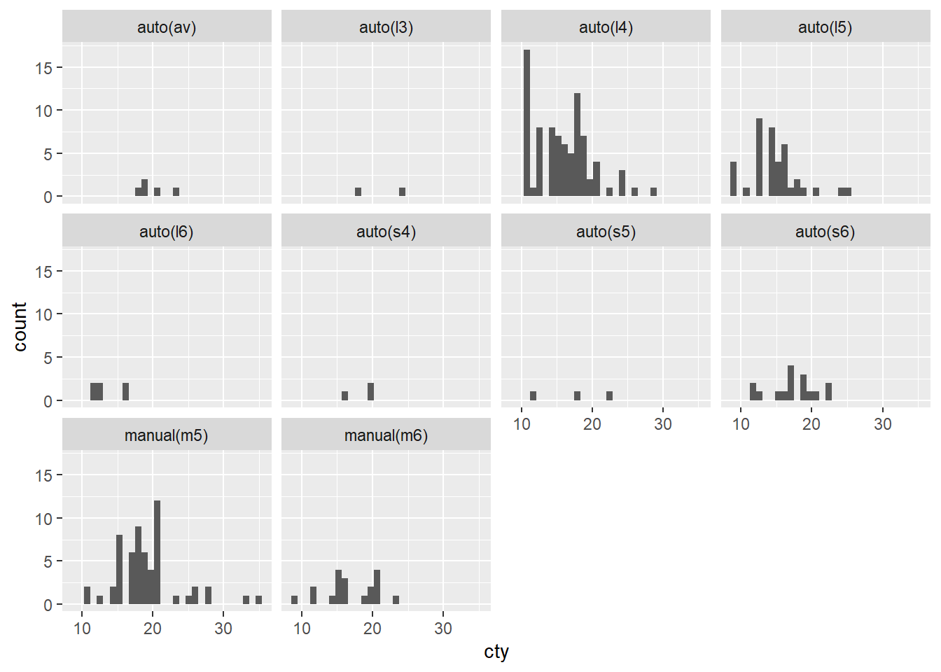
14.4 ggplot answers

14.4.1 Boxplot of highway miles per gallon versus class (mpg dataset)

Here is one possible solution:

mpg |> 
  ggplot(aes(x = class, y = hwy)) +
  geom_boxplot()

A prettier solution might be:

mpg |> 
  ggplot(aes(x = reorder(class, -hwy), y = hwy)) +
  geom_boxplot() +
  labs (x = "Car class",
        y = "Highway miles per gallon") +
  theme_classic()

14.4.2 Histogram of city miles per gallon faceted by transmission type (mpg dataset)

A possible solution:

mpg |> 
  ggplot(aes(x = cty)) +
  geom_histogram() +
  facet_wrap(facets = ~ trans)

14.5 Proof of variance

If we take our coos dataset again and create a new variable taking each value away from the mean:

distances <- coos |> 
  mutate(distances = mean(weight)-weight)

distances

## # A tibble: 12 × 3
##    heifer_id weight distances
##        <dbl>  <dbl>     <dbl>
##  1         1   211.    -0.683
##  2         2   200.    10.2  
##  3         3   220.    -9.48 
##  4         4   201.     9.82 
##  5         5   222    -11.4  
##  6         6   209.     1.32 
##  7         7   196.    14.8  
##  8         8   220.    -9.78 
##  9         9   225.   -14.6  
## 10        10   219.    -8.08 
## 11        11   194.    16.9  
## 12        12   210.     0.917

And then we add all the distances together . . .

round(sum(distances$distances), digits = 1)

## [1] 0

14.6 Tidy Unicorns

We can tidy our Unicorn dataset with the pivot_longer command:

RadioTidy <- Radio |> 
  pivot_longer(cols = c(NoRadio:RadioDiscussion),
               names_to = "Radio",
               values_to = "DustYield")