Chapter 11 How to choose your stats
This chapter is potentially controversial. I deliberately haven’t discussed statistics in great detail in this book, not least because I feel I re-learn stats every few years. This chapter is not setting out to teach you statistics. There are many statistical assumptions and issues that I breeze past in this chapter. In this chapter I want to give you a quick reference to running statistical analyses in R, and, importantly, interpreting those results.
A much, much better book is Andy Field, Jeremy Miles, and Zoe Field’s brilliant Discovering Statistics Using R book.
You can skip this chapter if:
- You are comfortable deciding which statistical test to use
So its happened. You’ve collected your data, you’ve installed R, and now you’re ready to run some analyses! But what on earth do you do next? How do you choose and interpret the right statistic?
To be brutally honest, only repeated practice and engaging with statistics can help build this skill, and the more you learn, the more uncertain you may feel! But what this chapter can do is to give you a bit of a cheat sheet and show you the ‘greatest hits’ of statistical testing in R. I will also use the APA 7th Edition Numbers and Statistics guide to report the statistical tests, and show you how to extract that information from the output, but you should also look up the style guide of your desired report (e.g. APA 7th Edition).
For this chapter I will use in-built R datasets and fake datasets to demonstrate these tests. I will also use the tidyverse package throughout (which offers a few more datasets), so you will want to have that loaded.
I will note here all the packages that are used in this chapter, and
highlight them at their specific tests. Remember, you can always install
a package with install.packages(“package_name”)
-
library(tidyverse) -
library(vcd) -
library(broom) -
library(pgirmess) -
library(clinfun)
11.1 Where to start
To work your way through this chapter, you need to identify your:
Response variable (the y axis)
Explanatory variable (the x axis)
and then work your way down this handy list:
I have a . . .
11.2 My response is a categorical variable
11.2.1 Categorical Response, Historical/Known Comparisons
11.2.1.1 Proportion of responses different from a known/expected result (1 Sample Proportion Test)
Our Data
Let’s say we have 20 German Shepherd dogs, and we know that the prevalence of hip dysplasia, a very painful condition, is usually 18% in this breed. We want to know if these particular dogs (perhaps they are from a new genetic line) are showing less hip dysplasia than we would expect. We have recorded whether or not these dogs are showing signs of dysplasia as a ‘yes/no’ categorical variable, and 3 dogs are showing signs of hip dysplasia.
We can run a 1 proportion test like so:
##
##  Exact binomial test
##
## data:  3 and 20
## number of successes = 3, number of trials = 20, p-value = 1
## alternative hypothesis: true probability of success is not equal to 0.18
## 95 percent confidence interval:
##  0.03207094 0.37892683
## sample estimates:
## probability of success
##                   0.15
Note that we don’t even need any real ‘data’ to run this test - its simply drawn from statistical probabilities. We would write this up as:
In this study, 15% of the dogs presented with signs of hip dysplacia, which is not significantly different from the historical prevalence of 18% in a binomial test (95% CI [3%-38%], p > .9).
What if we had more dogs?
We’ve continued running this study, mainly because we’re worried that only having 20 dogs is not accounting for enough of the natural variation we see in the world. This time we have 50 dogs from this genetic line and we’ve seen 4 of them develop dysplasia. As we have more than 30 responses, we can use a different version of the test.
##
##  1-sample proportions test with continuity correction
##
## data:  4 out of 50, null probability 0.18
## X-squared = 2.7439, df = 1, p-value = 0.09763
## alternative hypothesis: true p is not equal to 0.18
## 95 percent confidence interval:
##  0.0259402 0.2011004
## sample estimates:
##    p
## 0.08
This time we have a little more information that we can report with:
In this study, 8% of the dogs presented with hip dysplasia, which is not significantly different from the historical prevalence of 18% in a one sample proportion test (95% CI[3%-20%], X2 = 2.74, p = .098)
11.2.2 Categorical Response, Categorical Explanatory
11.2.2.1 Categorical Response (Repeated Measures) Categorical Explanatory, McNemar’s Test
Our Data
We have 40 German Shepherd dogs, some of whom already present with dysplasia, a painful condition. We’re concerned that after a season of work more dogs will develop dysplasia, and want to see if this is true. For this dataset we will create a contingency table:
work <- matrix(c(2, 5, 38, 35),
              ncol=2,
              byrow=TRUE,
              dimnames = list(c("Dysplasia", "No Dysplasia"),
                              c("Before Work Season", "After Work Season")))
We are going to run a specific test which accounts for the fact we have the same dogs in both conditions (before and after work):
##
##  McNemar's Chi-squared test with continuity correction
##
## data:  work
## McNemar's chi-squared = 23.814, df = 1, p-value = 1.061e-06
After the work season significantly more dogs developed dysplasia in McNemar’s test (X2[1, n = 40] = 23.81, p = <.001)
11.2.2.2 Proportion of responses compared across groups (Fishers/Chi2 test)
11.2.2.2.1 Fisher’s Exact Test (Small Sample Sizes / Summarised Data)
Our Data
German Shepherd Dogs suffer from hip dysplasia, a very painful condition. We know that more inbred dogs are more susceptible, and so we have followed 20 highly inbred dogs and 20 less inbred dogs and observed whether they developed the disease or not. As the prevalence is low (18% historically), we would not expect more than 3.6 dogs to develop dysplasia in either category (if it was left up to chance). For this reason, we should use Fisher’s Exact Test, which is more robust for smaller sample sizes.
Of the inbred dogs, we’ve seen 4 cases of dysplasia. Of the less inbred dogs, we’ve seen 2 cases of dysplasia. Like before, we can test this without having any actual data in R:
##
##  Fisher's Exact Test for Count Data
##
## data:  c(4, 16) and c(2, 18)
## p-value = 1
## alternative hypothesis: true odds ratio is not equal to 1
## 95 percent confidence interval:
##  0.02564066        Inf
## sample estimates:
## odds ratio
##        Inf
We do need to calculate one more thing to add to our report,the odds ratio:
## [1] 1.222222And this is reported like so:
A Fisher’s Exact Test found no significant difference in the frequency of dysplasia occurring in highly inbred dogs versus less inbred dogs (OR = 1.2, 95% CI[0.02-Inf], p > .9)
11.2.2.2.2 Chi2 Test (Larger Sample Sizes)
Our Data
This time we have observed more German Shepherd Dogs, a highly inbred line which we think will be more prone to hip dysplasia, and a less inbred line which we think will be less prone to hip dysplasia. For this dataset we will create a contingency table:
gsd <- matrix(c(16, 12, 84, 86),
              ncol=2,
              byrow=TRUE,
              dimnames = list(c("Dysplasia", "No Dysplasia"),
                              c("Inbred", "Less Inbred")))
With a Chi2 test we often also want to calculate an effect size, and there’s a handy package (vcd) which we can use to calculate Cramer’s V. We’ll calculate it here too. To interpret V, a small effect size is <0.10, a medium effect size < 0.30, and a large effect size is <0.50.
##
##  Pearson's Chi-squared test with Yates' continuity correction
##
## data:  gsd
## X-squared = 0.30714, df = 1, p-value = 0.5794## [1] 1.0625## X^2 df P(> X^2)
## Likelihood Ratio 0.57672 1 0.44760
## Pearson 0.57481 1 0.44835
##
## Phi-Coefficient : 0.054
## Contingency Coeff.: 0.054
## Cramer's V : 0.054And report like so:
A Chi2 test found no significant different in the frequency of dysplasia occurring in highly inbred dogs versus less inbred dos (OR 1.06, X2[1, n = 198] = 0.307, V = .05, p = .579)
11.2.3 Categorical Response, Numerical Explanatory (Logistic Regression)
Logistic regression is a bit of a ‘catch-all’ phase, certainly in this chapter. It’s also having its own day in the sun and is now often called a form of machine learning. I have mixed feelings about this that we can’t get into right now.
If you’re reading this chapter from top-to-bottom, this subheading will feel like a huge jump in difficulty. It is. We are beginning to step into the land of generalised linear models which are powerful statistical tools. If you’re very new to statistics and this is where your path has led you, you should really seek out advice from others. This is getting into the fun, meaty parts of statistical theory. But I did say I’d walk you through it . . .
Our Data
We have 21 German Shepherd Dogs. We took a measure of inflammation from their bodies, and then later recorded whether or not they were showing signs of hip dysplasia. We want to see if inflammation (a numerical score) can be used to predict whether the dogs will end up with hip dysplasia (a categorical variable, 0 = no signs, 1 = hip dysplasia).
We will need to generate this data in R:
dysp <- tibble(dysplasia = c(1, 1, 1, 1, 1, 1, 1,
                              0, 0, 0, 0, 0, 0, 0,
                              0, 0, 0, 0, 0, 0, 0),
                inflammation =c(0.91, 0.79, 1.40, 0.71, 1.01, 0.77, 0.85,
                                0.42, 1.02, 0.31, 0.05, 1.17, 0.04, 0.36,
                                0.12, 0.02, 0.05, 0.42, 0.92, 0.72,  1.05))
To run a binary logistic regression (predicting yes vs no from a numerical variable) we can use the glm command. We do need to take a few extra steps. For reporting we’ll also make use of the broom package.
##
## Call:
## glm(formula = dysplasia ~ inflammation, family = "binomial",
##     data = dysp)
##
## Deviance Residuals:
##     Min       1Q   Median       3Q      Max
## -1.5715  -0.5727  -0.3094   1.0397   1.4914
##
## Coefficients:
##              Estimate Std. Error z value Pr(>|z|)
## (Intercept)    -3.190      1.484  -2.150   0.0316 *
## inflammation    3.488      1.740   2.004   0.0450 *
## ---
## Signif. codes:  0 '***' 0.001 '**' 0.01 '*' 0.05 '.' 0.1 ' ' 1
##
## (Dispersion parameter for binomial family taken to be 1)
##
##     Null deviance: 26.734  on 20  degrees of freedom
## Residual deviance: 20.534  on 19  degrees of freedom
## AIC: 24.534
##
## Number of Fisher Scoring iterations: 5## 'log Lik.' -10.26719 (df=2)## OddsRatio 2.5 % 97.5 %
## (Intercept) 0.04118154 0.0008355444 0.4146414
## inflammation 32.71638289 1.9151146706 2735.6121035And we could report this like so:
For each unit increase in inflammation, the odds of developing hip dysplasia increases by a factor of 32.7 in a binary logistic regression (Table 11.1)
library(broom)

tidy(logit) |>
  mutate(OddsRatio = exp(coef(logit))) |>
  select(term, estimate, std.error, statistic, OddsRatio, p.value ) |>
kable(caption = "Coefficient table for variables in binary logistic regression predicting hip dysplasia\nfrom inflammation markers in 21 German Shepard Dogs")| term | estimate | std.error | statistic | OddsRatio | p.value |
|---|---|---|---|---|---|
| (Intercept) | -3.189765 | 1.48362 | -2.149988 | 0.0411815 | 0.0315561 |
| inflammation | 3.487876 | 1.74028 | 2.004204 | 32.7163829 | 0.0450482 |
If you want to dig more deeply into logistic regressions, or model more predictor variables, I think this link is good. Remember to talk to your nearest friendly statistician.
11.3 My response is a numerical variable
11.3.1 Numerical Response, Historical/Known Comparisons (One Sample t-Test)
Our Data
The dataset trees gives us the height in feet of 31 black cherry trees. We want to know if these trees differ from a historical average height of 80ft. The t test command in R is simplistic, and so we do need to calculate the mean of height (mu) in addition to the t test to report properly.
##
##  One Sample t-test
##
## data:  trees$Height
## t = -3.4952, df = 30, p-value = 0.001496
## alternative hypothesis: true mean is not equal to 80
## 95 percent confidence interval:
##  73.6628 78.3372
## sample estimates:
## mean of x
## 76## mean sd
## 1 76 6.371813We would report this like so:
The mean height (76ft +/- 6.37) for black cherry trees was smaller than the historical average of 80ft in a one-sample t-test (t(30) = -3.50, p = .001)
11.3.2 Numerical Response (Repeated Measures), Categorical Explanatory (Paired t-Test)
Our Data
In this example we have 10 housecats who we put on a special weight-loss diet. We weigh them before the diet and after, and we want to see if they have lost any weight. We can do this with a paired t-test.
diet <- tibble (before = c(5.04, 4.63, 4.04, 5.10, 5.43, 4.83, 3.45, 3.49, 5.02, 4.81),
                after = c( 4.78, 2.49, 4.46, 2.03, 5.13, 7.23, 3.50, 1.89, 3.30, 3.91))

diet |>
  summarise(b_mean = mean(before),
            a_mean = mean(after),
            b_sd = sd(before),
            a_sd = sd(after))
## # A tibble: 1 × 4
## b_mean a_mean b_sd a_sd
## <dbl> <dbl> <dbl> <dbl>
## 1 4.58 3.87 0.689 1.62##
## Paired t-test
##
## data: diet$before and diet$after
## t = 1.4615, df = 9, p-value = 0.1779
## alternative hypothesis: true mean difference is not equal to 0
## 95 percent confidence interval:
## -0.3900511 1.8140511
## sample estimates:
## mean difference
## 0.712After being on the weight-loss diet, cats weighed 3.9kg (+/- 1.62kg SD), compared to a mean weight of 4.6kg (+/- 0.69kg SD) before going on the diet, but this difference of 0.71kg (95% CI [-0.39, 1.81]) was not statistically significant in a paired t-test (t(9) = 1.46, p = .178)
11.3.3 Numerical Response, Categorical Explanatory (ANOVA/GLM)
Traditionally, depending on how many explanatory variables you have and whether your design is balanced or unbalanced, you would select a different type of test, leading up to a general linear model as the most flexible form.
One explanatory factor = 1 way ANOVA
Two explanatory factors and balanced design = 2-way ANOVA
Three or more explanatory factor or unbalanced design = general linear model (glm)
I like using the Grafen and Hails approach to statistics, and considering all ANOVAs to be a glm. I am fundamentally lazy, and don’t like to remember three separate things when one model will do it all for me. Real statisicians may cry at this.
Our data
Let’s use the chickwts data to explore this. chickwts describes a simple experiment with six different feedtypes and the weights of the chicks fed on them. We are looking for the feedtype which provides the heaviest chick on average.
As an ANOVA
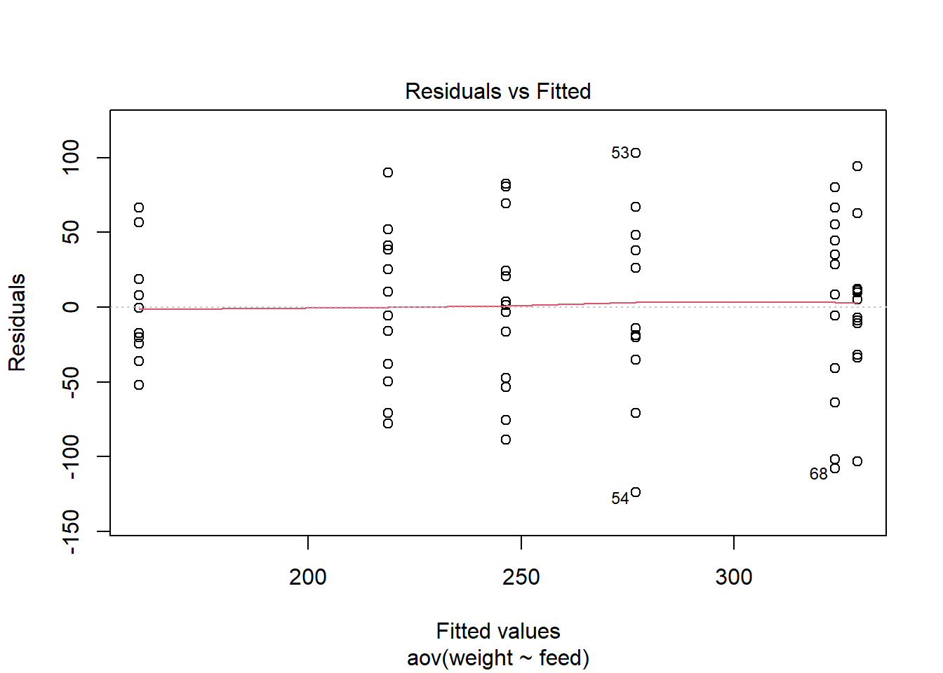
The basic steps of running a one-way ANOVA test is to create the model, inspect the model, check the model assumptions with a residual plot, and run pairwise comparisons to define the difference between the levels. Its also very difficult to interpret this without a plot so we’ll add on of those to our interpretation.
##             Df Sum Sq Mean Sq F value   Pr(>F)
## feed         5 231129   46226   15.37 5.94e-10 ***
## Residuals   65 195556    3009
## ---
## Signif. codes: 0 '***' 0.001 '**' 0.01 '*' 0.05 '.' 0.1 ' ' 1## Tukey multiple comparisons of means
## 95% family-wise confidence level
##
## Fit: aov(formula = weight ~ feed, data = chickwts)
##
## $feed
## diff lwr upr p adj
## horsebean-casein -163.383333 -232.346876 -94.41979 0.0000000
## linseed-casein -104.833333 -170.587491 -39.07918 0.0002100
## meatmeal-casein -46.674242 -113.906207 20.55772 0.3324584
## soybean-casein -77.154762 -140.517054 -13.79247 0.0083653
## sunflower-casein 5.333333 -60.420825 71.08749 0.9998902
## linseed-horsebean 58.550000 -10.413543 127.51354 0.1413329
## meatmeal-horsebean 116.709091 46.335105 187.08308 0.0001062
## soybean-horsebean 86.228571 19.541684 152.91546 0.0042167
## sunflower-horsebean 168.716667 99.753124 237.68021 0.0000000
## meatmeal-linseed 58.159091 -9.072873 125.39106 0.1276965
## soybean-linseed 27.678571 -35.683721 91.04086 0.7932853
## sunflower-linseed 110.166667 44.412509 175.92082 0.0000884
## soybean-meatmeal -30.480519 -95.375109 34.41407 0.7391356
## sunflower-meatmeal 52.007576 -15.224388 119.23954 0.2206962
## sunflower-soybean 82.488095 19.125803 145.85039 0.0038845We first inspect the plot to ensure the residuals are normally distributed. If we saw a pattern here we would know that the model is consistently underfitting or overfitting some observations, and that one of the ANOVA’s key assumptions had not been met (in this case there are many future options but you really should be talking to a statistician or friendly peer at this point).
There was a significant effect of feedtype on chick weight in a one-way ANOVA (F(5,65) = 15.37, p <.001, Figure 11.1). Post-hoc comparisons with Tukeys HSD found variety in performance, with sunflower feeds significantly outperformed soybean (82g, p = .003) linseed (110g, p <.001), and horsebean (168g, p <.001). Casein diets outperform horsebean (163g, p <.001), linseed (105g, p <.001), and soybean (77g, p = .008). Meatmeal outperforms horsebean (117g, p <.001) and soybean outperformed horsebean (86g, p = .004).
chickwts |>
  ggplot(aes(x = reorder(feed, -weight), y = weight)) +
  geom_boxplot()+
  theme_classic() +
  labs(y = "Weight (g)",
       x = "Feedtype")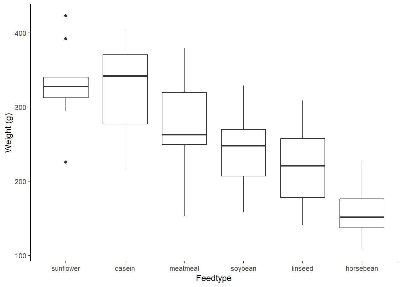
Figure: 11.1: Chick weight (g) per feed type, data from ‘chickwts’
As a linear model
The lm argument fits linear models and can do ANOVAs and regressions. Its my preferred way of running this kind of analysis, partly because I think the R2 number (a measure of how good a ‘fit’ the model is) is a really useful way to help present the data. We can also use the broom package for extra reporting and to visualise effects.
##
## Call:
## lm(formula = weight ~ feed, data = chickwts)
##
## Residuals:
##      Min       1Q   Median       3Q      Max
## -123.909  -34.413    1.571   38.170  103.091
##
## Coefficients:
##               Estimate Std. Error t value Pr(>|t|)
## (Intercept)    323.583     15.834  20.436  < 2e-16 ***
## feedhorsebean -163.383     23.485  -6.957 2.07e-09 ***
## feedlinseed   -104.833     22.393  -4.682 1.49e-05 ***
## feedmeatmeal   -46.674     22.896  -2.039 0.045567 *
## feedsoybean    -77.155     21.578  -3.576 0.000665 ***
## feedsunflower    5.333     22.393   0.238 0.812495
## ---
## Signif. codes:  0 '***' 0.001 '**' 0.01 '*' 0.05 '.' 0.1 ' ' 1
##
## Residual standard error: 54.85 on 65 degrees of freedom
## Multiple R-squared:  0.5417, Adjusted R-squared:  0.5064
## F-statistic: 15.36 on 5 and 65 DF, p-value: 5.936e-10library(broom)
chk_l |>
tidy() |>
ggplot(aes(x = reorder(term, - estimate), y = estimate)) +
geom_point(aes(colour = term, shape = term)) +
geom_errorbar(aes(x = term, ymin = estimate-std.error, ymax = estimate+std.error, colour = term)) +
theme_classic()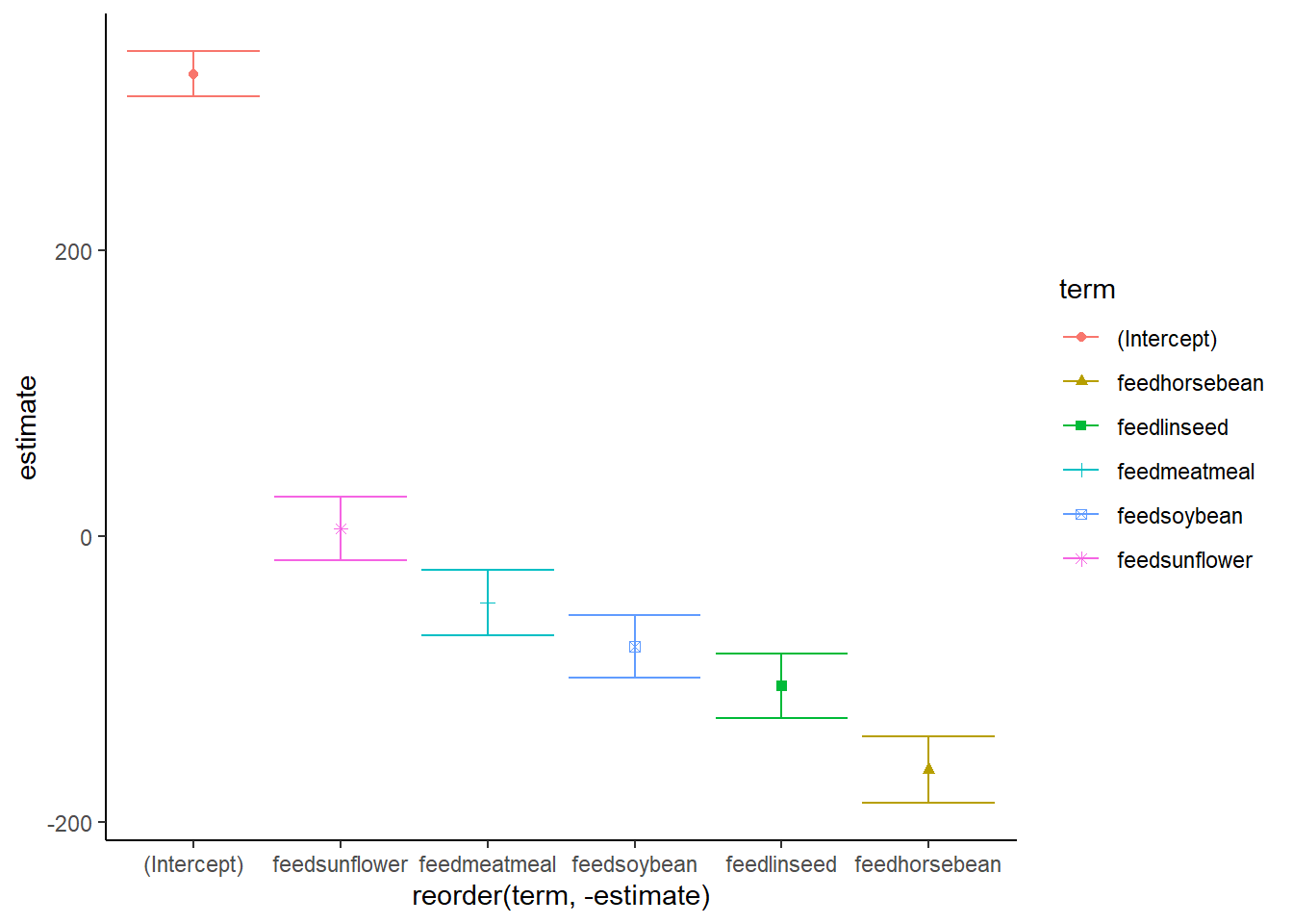
Feedtype had a significant effect in a linear model, explaining 51% of the variance observed in chick weight. (F(5,65) = 15.36, p < .001). Meatmeal had a moderately lower weight gain than casein (t = -2.04 p = .046), soybean (t = -3.58, p = < .001), linseed (t = -4.68, p < .001), and horsebean (t = -6.96, p <.001) all had much lower weight gains. There was no significant difference between the casein diet and the sunflower diet (t = 0.24, p = .812).
11.3.4 Numerical Response, Numerical Explanatory (Correlation & Regression)
Our data
We will use the trusty cars dataset which describes the speed (mph) and stopping distance (ft) of cars in the 1920s to talk about two types of test, Pearson’s correlation and linear regression.
As Pearson’s correlation
As many, many, many folk say, correlation is not causation. In statistical terms, that means that correlation does not aim to predict y from x, only to see if there is an underlying structure to the variation.
##
##  Pearson's product-moment correlation
##
## data:  cars$speed and cars$dist
## t = 9.464, df = 48, p-value = 1.49e-12
## alternative hypothesis: true correlation is not equal to 0
## 95 percent confidence interval:
##  0.6816422 0.8862036
## sample estimates:
##       cor
## 0.8068949
Speed has a strong, positive association with the stopping distance of cars in a correlation (r = .81, 95%CI[.68, .89], t(48) = 9.46, p <.001).
As a regression
In a linear model, we can be more definitive in our reporting.
##
## Call:
## lm(formula = dist ~ speed, data = cars)
##
## Residuals:
##     Min      1Q  Median      3Q     Max
## -29.069  -9.525  -2.272   9.215  43.201
##
## Coefficients:
##             Estimate Std. Error t value Pr(>|t|)
## (Intercept) -17.5791     6.7584  -2.601   0.0123 *
## speed         3.9324     0.4155   9.464 1.49e-12 ***
## ---
## Signif. codes:  0 '***' 0.001 '**' 0.01 '*' 0.05 '.' 0.1 ' ' 1
##
## Residual standard error: 15.38 on 48 degrees of freedom
## Multiple R-squared:  0.6511, Adjusted R-squared:  0.6438
## F-statistic: 89.57 on 1 and 48 DF,  p-value: 1.49e-12
Stopping distance increased by 3.9ft for every mph faster the car travelled at (R2 = 64%, F(1,48) = 89.6, p<.001)
11.4 My response is an ordinal variable
11.4.1 Ordinal Response, Historical/Known Comparisons (One Sample Wilcoxan Test)
Our data
In this example we have student ratings of this textbook from 1 (very unsatisfied) to 5 (very satisfied). We’re hoping that at the very least, people are satisfied, and have ranked the book a 4. For this we can use the One Sample Wilcoxan Test, but we need to calculate an additional step, the median.
ratings <- tibble(satisfaction = c(1,2,1,1,3,2,1,5,1,2,5,1,2,3,3,1,3))

ratings |>
  summarise(median = median(satisfaction))
## # A tibble: 1 × 1
## median
## <dbl>
## 1 2##
## Wilcoxon signed rank test with continuity correction
##
## data: ratings$satisfaction
## V = 7, p-value = 0.0009212
## alternative hypothesis: true location is not equal to 4The textbook achieved a medium score of ‘2’, or ‘unsatisfied’ from students, which was significantly lower than the desired median score of ‘4’ or ‘satisfied’ in a one-sample Wilcoxan test (V = 7, p = <.001).
11.4.2 Ordinal Response (Repeated Measures), Categorical Explanatory (One Sample Wilcoxan Signed-Rank Test)
Our data
In this example we have student ratings of this textbook from 1 (very unsatisfied) to 5 (very satisfied). We made some changes to the book after the first set of reviews and we’re hoping the same students will now score the book higher. For this we can use the Wilcoxan Signed Rank Test, but we need to calculate an additional step, the median.
ratings <- tibble(satisfaction1 = c(1,2,1,1,3,2,1,5,1,2,5,1,2,3,3,1,3),
                  satisfaction2 = c(1,4,2,3,3,3,2,5,2,4,5,3,3,3,4,1,3))

ratings |>
  summarise(satis1 = median(satisfaction1),
            satis2 = median(satisfaction2))
## # A tibble: 1 × 2
## satis1 satis2
## <dbl> <dbl>
## 1 2 3wilcox.test(x = ratings$satisfaction1, ratings$satisfaction2, paired = TRUE, alternative = "two.sided")##
## Wilcoxon signed rank test with continuity correction
##
## data: ratings$satisfaction1 and ratings$satisfaction2
## V = 0, p-value = 0.004565
## alternative hypothesis: true location shift is not equal to 0After revisions, the textbook received a median score of ‘3’ (undecided), which was significantly higher than the before revision median score of ‘2’ (unsatisfied) in a Wilcoxan Signed Rank Test (V = 0, p = .005).
11.4.3 Ordinal Response, Categorical Explanatory
Our data
In this example, we have measured student satisfaction with their R teaching on a 5-point scale from 1 (very unsatisfied) to 5 (very satisfied). We have three conditions, students who searched their own materials (self-taught), students who received this textbook (textbook), and students who received the textbook plus tutorials (textbook plus). We want to know which students were most satisfied. For this we can use a Kruskal-Wallis test. We can use two more functions, kruskalmc from library(pgirmess) and jonckheere.test from library(clinfun) to help us interpret the data. Jonkheere-Terpstra tests are technically a different type of test, but are useful in exploring how ordered differences occur, e.g. in this case we expect that each intervention will improve student satisfaction, and that textbook-plus will be better than textbook, which itself will be better than self-taught.
library(clinfun)
library(pgirmess)

textbk <- tibble(self_taught = c(1,2,1,1,3,2,1,5,1,2,5,1,2,3,3,1,3),
                 textbook= c(1,4,2,3,3,3,2,5,2,4,5,3,3,3,4,1,3),
                 textbook_plus = c( 3, 2, 3, 3, 3, 3, 2, 4, 4, 5, 3, 4, 4, 5, 4, 5, 3)) |>
  pivot_longer(cols = c(self_taught:textbook_plus),
               names_to = "condition",
               values_to = "score")


kruskal.test(score ~ condition, textbk)
##
## Kruskal-Wallis rank sum test
##
## data: score by condition
## Kruskal-Wallis chi-squared = 10.503, df = 2, p-value = 0.00524## Multiple comparison test after Kruskal-Wallis, treatments vs control (two-tailed)
## alpha: 0.05
## Comparisons
## obs.dif critical.dif stat.signif
## self_taught-textbook 9.705882 11.42896 FALSE
## self_taught-textbook_plus 15.882353 11.42896 TRUE##
## Jonckheere-Terpstra test
##
## data:
## JT = 616, p-value = 0.001609
## alternative hypothesis: two.sidedStudent satisfaction increased significantly with intervention (H(2) = 10.5, p* = .005), with textbook-plus showing a significant difference (p<.05) from self-taught, but no difference between self-taught and textbook (p>.05). The directionality of effect was significant in a Jonckheere-Terpstra test (T = 616, p = .002, Figure 11.2)
textbk |>
  ggplot(aes(x = condition, y = score)) +
  geom_boxplot()+
  theme_classic() +
  scale_y_continuous(breaks = seq(1,5,1), limits = c(1,5), labels = c("Very unsatisfied", "Unsatisfied", "Not sure",
                                                                  "Satisfied", "Very satisfied")) +
  scale_x_discrete(labels = c("Self-Taught", "Textbook", "Textbook plus lecture")) +
  labs(x = "Teaching Method", y = "Score")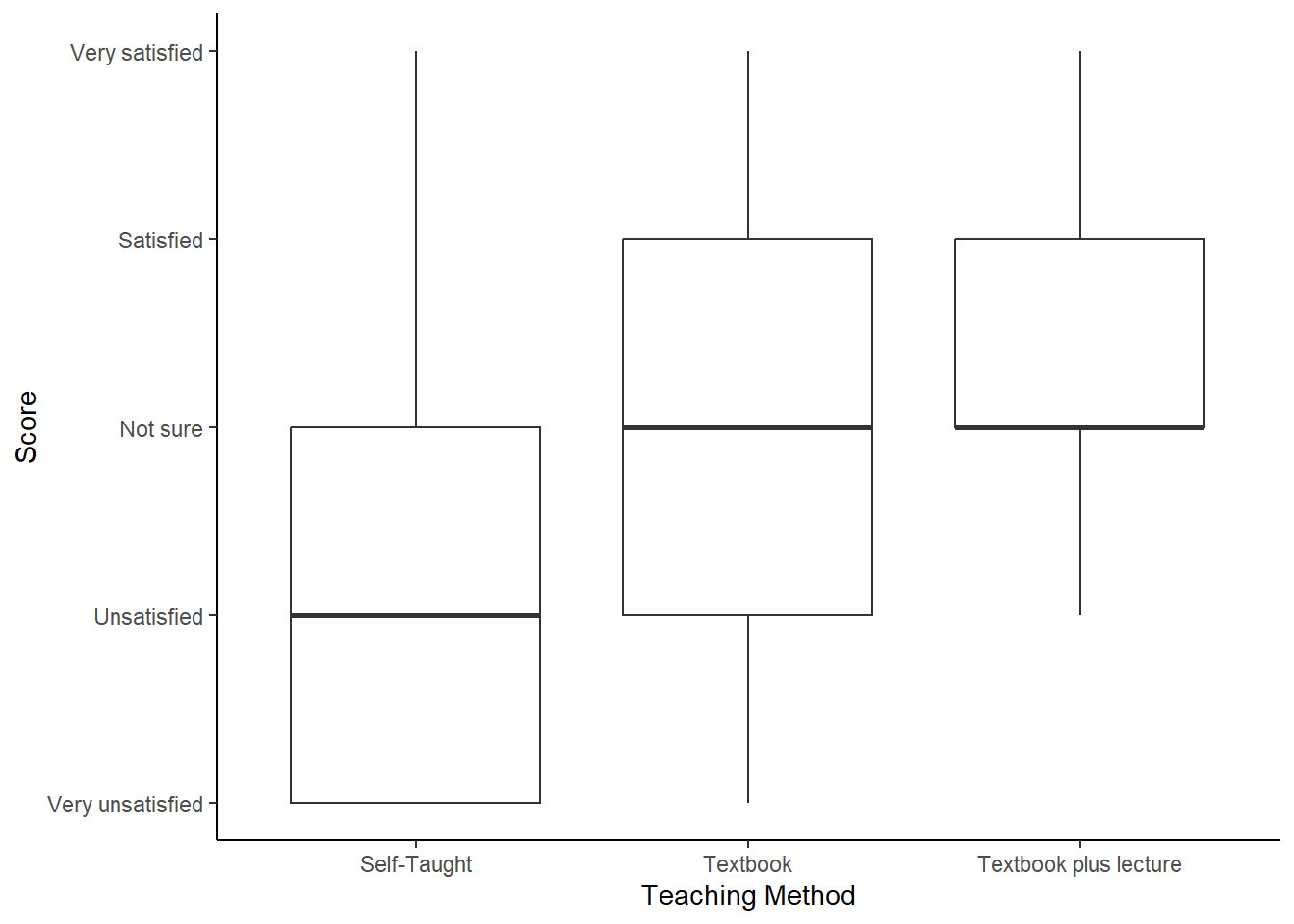
Figure: 11.2: Student satisfaction by teaching method
11.4.4 Ordinal Response, Numerical Explanatory (Spearman rank correlation)
Our data
When you have an ordinal response and either a numerical explanatory or an ordinal explanatory variable, a Spearman rank correlation is probably for you. A Spearman rank correlation is exactly the same as a Pearson correlation, but the data is ranked (or ordered) before the calculation is run. Spearman rank correlations are therefore often used for skewed data.
Let’s say we have 15 students who have ranked their satisfaction with the course (from 1, “Very unsatisfied” to 5, “Very satisfied”) and their grades (E, “very poor”, to A “excellent”). We think students who are very satisfied will have higher grades.
grades <- tibble(satisfaction = c(1, 5, 2, 1, 1, 5, 4, 5, 4, 5, 5, 3, 4, 3, 1),
                 grade = c(1, 4, 1,2, 1, 4, 5, 5, 5, 4, 3, 3, 2, 2,1 ))

cor.test(grades$satisfaction, grades$grade,method = "spearman")
##
## Spearman's rank correlation rho
##
## data: grades$satisfaction and grades$grade
## S = 121.25, p-value = 0.0005493
## alternative hypothesis: true rho is not equal to 0
## sample estimates:
## rho
## 0.7834775Student satisfaction was strongly positively associated with grade (rs = .78,p<.001)