5  Week 4: Considerations for Collecting Data

Lecture: Effect Sizes and Covariance

Mock Data and visualisation

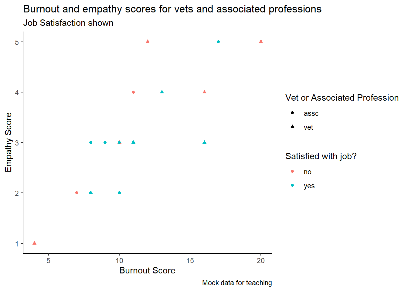
job_dat <- tibble(job = c("vet", "vet", "vet","vet", "vet", "vet", "vet", "vet", "vet", "vet",
                          "assc", "assc", "assc", "assc", "assc", "assc", "assc", "assc", "assc", "assc"),
                  burnout = c(13, 12, 4, 16, 16, 20, 8, 10, 11, 10,
                              10, 11, 8, 7, 8, 10, 9, 11, 17, 10),
                  empathy = c(4, 5, 1, 4,3, 5, 2, 3,3,2,
                              2, 3, 3, 2, 2, 3, 3, 4, 5, 2),
                  satisfaction = c("yes", "no", "no", "no", "yes", "no", "yes", "no", "yes", "yes",
                                   "yes", "yes", "yes", "no", "yes", "yes", "yes","no", "yes", "yes"))


job_dat |> 
  ggplot(aes(x = burnout, y = empathy, shape = job, colour = satisfaction)) +
  geom_point() +
  theme_classic() +
  labs(title = "Burnout and empathy scores for vets and associated professions",
       subtitle = "Job Satisfaction shown",
       caption = "Mock data for teaching",
       x = "Burnout Score",
       y = "Empathy Score") +
  scale_shape_discrete(name = "Vet or Associated Profession") +
  scale_color_discrete(name = "Satisfied with job?") 

Calculcate Cohen’s d

library(effsize)

cohen.d(d = job_dat$burnout, f = job_dat$job)

Cohen's d

d estimate: -0.5048995 (medium)
95 percent confidence interval:
     lower      upper 
-1.4593128  0.4495138 

Calculcate Hedge’s g

cohen.d(d = job_dat$burnout, f = job_dat$job, hedges.correction = TRUE)

Hedges's g

g estimate: -0.4835657 (small)
95 percent confidence interval:
     lower      upper 
-1.3964834  0.4293519 

Effects of Differences

job_dat |> 
  ggplot(aes(x = burnout, y = empathy)) +
  geom_point() +
  theme_classic() +
  labs(x = "Burnout Score", y = "Empathy Score")

Correlation coefficient (r)

cor(job_dat$burnout, job_dat$empathy, method = "pearson")

[1] 0.7991678

Other Correlation Coefficients

cor(job_dat$burnout, job_dat$empathy, method = "spearman")

[1] 0.8202187

cor.test(job_dat$burnout, as.numeric(as.factor(job_dat$job)))

    Pearson's product-moment correlation

data:  job_dat$burnout and as.numeric(as.factor(job_dat$job))
t = 1.129, df = 18, p-value = 0.2737
alternative hypothesis: true correlation is not equal to 0
95 percent confidence interval:
 -0.2091671  0.6281908
sample estimates:
      cor 
0.2571562 

Cramer’s V

library(lsr)

job_dat <- job_dat |> 
  mutate(burnoutcat = case_when(burnout > 10 ~ "burnout",
                                TRUE ~ "no burnout"))


job_tbl <- xtabs(~job_dat$job +  job_dat$satisfaction + job_dat$burnoutcat)
ftable(job_tbl)

                                 job_dat$burnoutcat burnout no burnout
job_dat$job job_dat$satisfaction                                      
assc        no                                            1          1
            yes                                           2          6
vet         no                                            3          2
            yes                                           3          2

chisq.test(ftable(job_tbl))

    Pearson's Chi-squared test

data:  ftable(job_tbl)
X-squared = 2.2222, df = 3, p-value = 0.5276

cramersV(ftable(job_tbl))

[1] 0.3333333

R²adj Example

jobmod <- lm(burnout ~ empathy + satisfaction, data = job_dat)
summary(jobmod)

Call:
lm(formula = burnout ~ empathy + satisfaction, data = job_dat)

Residuals:
    Min      1Q  Median      3Q     Max 
-3.7526 -1.0832 -0.3836  1.4822  4.7305 

Coefficients:
                Estimate Std. Error t value Pr(>|t|)    
(Intercept)       1.9944     1.8904   1.055    0.306    
empathy           2.7516     0.4865   5.656 2.85e-05 ***
satisfactionyes   1.0202     1.1393   0.895    0.383    
---
Signif. codes:  0 '***' 0.001 '**' 0.01 '*' 0.05 '.' 0.1 ' ' 1

Residual standard error: 2.354 on 17 degrees of freedom
Multiple R-squared:  0.6549,    Adjusted R-squared:  0.6144 
F-statistic: 16.13 on 2 and 17 DF,  p-value: 0.000118

job_dat |> 
  mutate(mod = predict(jobmod)) |> 
  ggplot() + 
  geom_point(aes(x = empathy, y = burnout, colour = satisfaction)) +
  geom_line(aes(x = empathy, y = mod)) +
  theme_classic() +
  facet_wrap(facets = ~ satisfaction, ncol = 1) +
  labs(x = "Empathy Score", y = "Burnout Score")

5.1 Covariance {. unnumbered}

jobmod2 <- lm(burnout ~ empathy + job, data = job_dat)
summary(jobmod2)

Call:
lm(formula = burnout ~ empathy + job, data = job_dat)

Residuals:
    Min      1Q  Median      3Q     Max 
-4.6359 -1.3894 -0.4212  1.6035  4.5151 

Coefficients:
            Estimate Std. Error t value Pr(>|t|)    
(Intercept)    2.631      1.552   1.695    0.108    
empathy        2.575      0.471   5.469 4.16e-05 ***
jobvet         1.127      1.052   1.072    0.299    
---
Signif. codes:  0 '***' 0.001 '**' 0.01 '*' 0.05 '.' 0.1 ' ' 1

Residual standard error: 2.331 on 17 degrees of freedom
Multiple R-squared:  0.6615,    Adjusted R-squared:  0.6217 
F-statistic: 16.61 on 2 and 17 DF,  p-value: 0.0001002

job_dat |> 
  mutate(mod = predict(jobmod2)) |> 
  ggplot() + 
  geom_point(aes(x = empathy, y = burnout, colour = job)) +
  geom_line(aes(x = empathy, y = mod)) +
  theme_classic() +
  facet_wrap(facets = ~ job, ncol = 1) +
  labs(x = "Empathy Score", y = "Burnout Score")